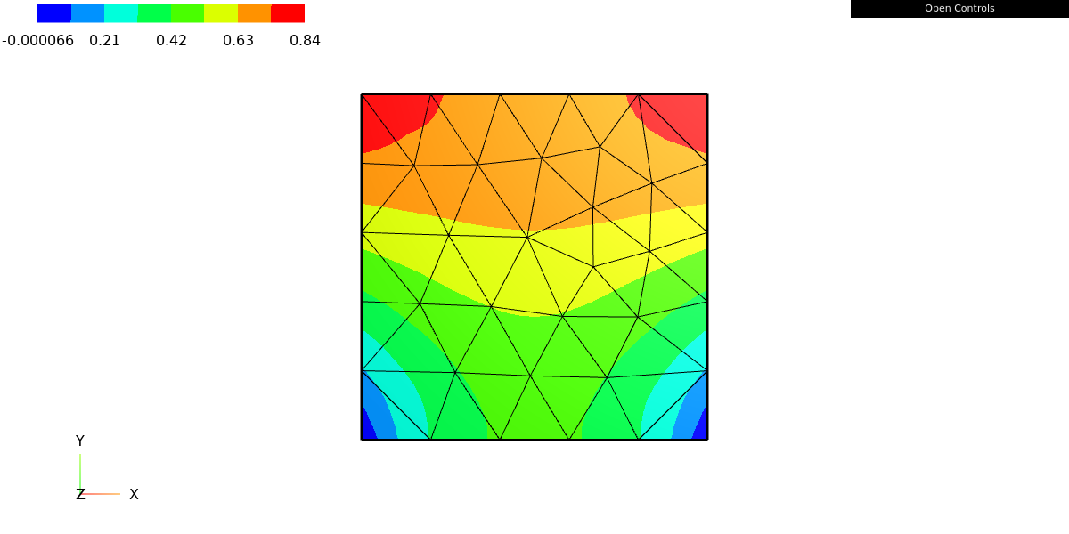
Solve for the free dofs¶

We need to assemble the right hand side of $A_{FF}u_{0,F}=f_F-\left[ Au_D \right]_F$, namely

r=f-Au_D

f = LinearForm(fes)
f += 1*v*dx
f.Assemble()

r = f.vec.CreateVector()
r.data = f.vec - a.mat * gfu.vec

This code creates a linear form f, and it represents the left hand side of the weak form of a PDE. In this case, a constant function 1 is used as a forcing term and multiplied by the trial function v and integrated over the domain using the dx measure.

f.Assemble() assembles the linear form, it performs the integration and the summation over the elements of the mesh. This step is required before solving a PDE.

The next line creates a new vector r which will store the result of the following operation f.vec - a.mat * gfu.vec. Here, f.vec represents the assembled version of the linear form f, a.mat represents the assembled version of the bilinear form a, and gfu.vec represents the current value of the grid function gfu. r.data = f.vec - a.mat * gfu.vec performs a matrix-vector multiplication between the assembled matrix of the bilinear form a and the current value of the grid function gfu, and it subtracts the result from the assembled version of the linear form f. The result is stored in the vector r.

This r vector is known as the residual vector, it is the difference between the left-hand side and the right-hand side of the discretized equation. It is typically used in the process of iteratively solving a PDE, such as the Newton-Raphson method, the residual is used to check if the solution is converging and to correct it if it is not.

gfu.vec.data += a.mat.Inverse(freedofs=fes.FreeDofs()) * r
Draw(gfu)

This code updates the current value of the grid function gfu by adding the solution to the linear system represented by a.mat * gfu.vec = f.vec.

The first part of the operation a.mat.Inverse(freedofs=fes.FreeDofs()) computes the inverse of the assembled matrix of the bilinear form a, it is used to solve the linear system. freedofs=fes.FreeDofs() is used to specify that only the free degrees of freedom of the solution, which are not constrained by any condition, should be considered while solving the system. This can be useful in cases where some degrees of freedom are known and fixed.

The second part *r computes the product of the inverse matrix by the residual vector. This product represent the update of the solution.

Then the solution update is added to the current value of the grid function gfu.vec.data +=

Finally, the last line Draw(gfu) is used to visualize the updated solution. As it is mentioned before, it will open a window with the solution graph, assuming the required visualization library is installed.