Extension of boundary data¶

We use the standard technique of reducing a problem with essential non-homogeneous boundary conditions to one with homogeneous boundary condition using an extension. The solution $u$ in $H_1$ satisfiesu$\Gamma_D=g$

and

\int_{\Omega} \nabla u \cdot \nabla v_0dV = \int_{\Omega}fv_0dV

for all $v_0$ in $\in H_{0,D}^1= { v \in H^1 : v|_{\Gamma_D} = 0 }$. Split the solution

u=u0+uD

where $u_D$ is an extension of $g$ into $\Omega$. Then we only need to find $u_0$ in $H_{0,D}^1 satisfying the homogeneous Dirichlet problem

\int_{\Omega} \nabla u_0 \cdot \nabla v_0 dV= \int_{\Omega}fv_0dV-\int_{\Omega} \nabla u_D \cdot \nabla v_0 dV

for all $v_0$ in $H_{0,D}^1$. These are the issues to consider in this approach:

• How to define an extension $u_D$ in the finite element space?
• How to form and solve the system for $u_0$?

Let us address the first in the following example.

Suppose we are given that

g=sin(y) \ \ \ \ \ \ \ \ \ \ on \ \  \Gamma_D

g=sin(y)

The code you provided creates a mathematical function g(y) = sin(y). This function represents the mathematical expression of sine of y, where y is a variable, and the output will be between -1 and 1.

It is possible to use this function as an input for some numerical computation as a forcing term for example for a differential equation or a functional, as long as it is defined on the domain of the problem.

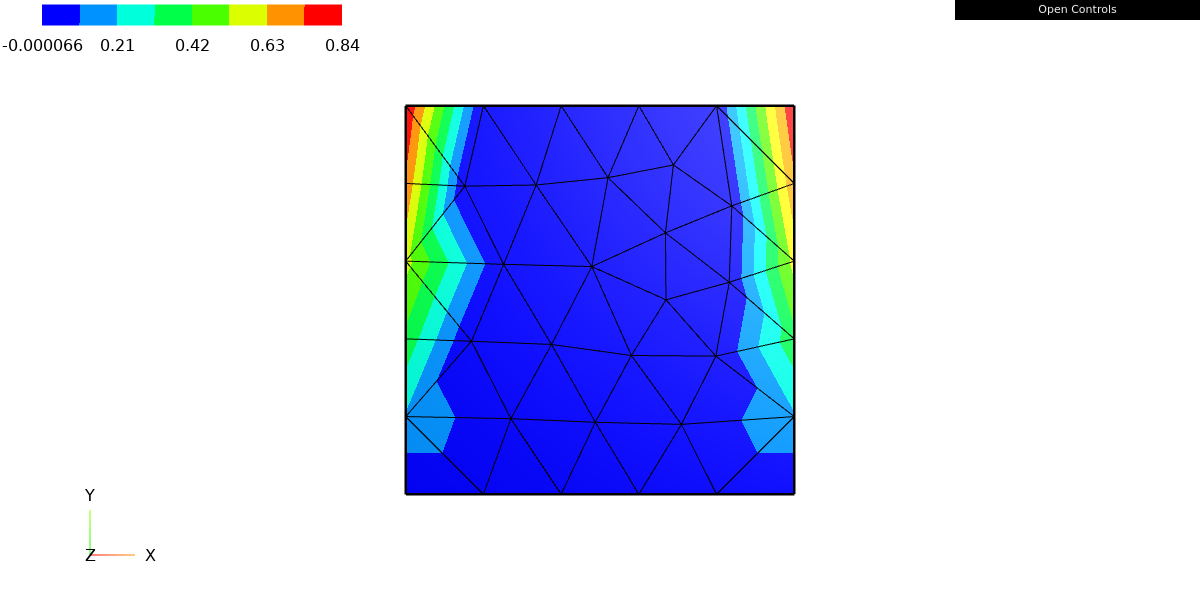
We interpolate g on the boundary of the domain and extend it to zero on the elements not having an intersection with \Gamma_D.

gfu = GridFunction(fes)
gfu.Set(g, BND)
Draw(gfu)

The first line creates a GridFunction object, gfu, which is a function defined over the finite element space fes previously defined. GridFunction is a class that represents a discrete function, such as the solution of a PDE or an initial condition, defined over a finite element space.

The second line gfu.Set(g, BND) sets the value of the GridFunction gfu to the function g on the boundary (BND) of the mesh. This means that the GridFunction gfu will take the value of the function g(y) = sin(y) on the boundary.

The third line, Draw(gfu), is used to visualize the solution. It will open a window with the solution graph.

Please note that this Draw method require visualization library like VisPy, PyVista, Matplotlib to be installed in your python environment. It is also important to specify that Draw is not the only way to visualize the solution, you can also use other library like Paraview to visualize your solution in 3D.

Forms and assembly¶

u, v = fes.TnT()
a = BilinearForm(fes, symmetric=True)
a += grad(u)*grad(v)*dx
a.Assemble()

The code you provided is defining a bilinear form a on the finite element space fes which is symmetric, by setting the symmetric=True attribute.

fes.TnT() function, stands for “test and trial space”, returns two finite element functions u and v which are in the same space as fes. These u and v functions are used as test and trial functions in the definition of the bilinear form.

The next line of the code, a += grad(u)*grad(v)*dx, defines the bilinear form a. The left-hand side of this equation is the bilinear form a, and the right-hand side is the integral over the domain of the product of the gradient of the test function u and the gradient of the trial function v (i.e. the weak form of Laplace operator). dx refers to the integration measure over the domain, in this case it means integrating over all the domain.

The last line of code, a.Assemble(), assembles the bilinear form, means it performs the integration and the summation over the elements of the mesh. Assembling a bilinear form means it converts it from a weak form to a matrix form and it is a required step before solving a PDE.

This assembled matrix (bilinear form) can be used as a part of a linear system of equations, which is typically used to solve PDEs.

#Result
<ngsolve.comp.BilinearForm at 0x7f4328de22f0>

If A= a.mat is the matrix just assembled, then we want to solve for

A(u_0+u_D)=f \Rightarrow Au_0=f-Au_D

or

\left[\begin{matrix}
A_{FF} & A_{FD} \\
A_{DF} & A_{DD} \\
\end{matrix}
\right]
\left[
\begin{matrix}
u_{0,F} \\
0
\end{matrix}
\right]
=
\left[
\begin{matrix}
f_F \\
f_D
\end{matrix}
\right]
-
\left[\begin{matrix}
A_{FF} & A_{FD} \\
A_{DF} & A_{DD} \\
\end{matrix}
\right]
\left[
\begin{matrix}
u_{D,F} \\
u_{D,D}
\end{matrix}
\right]

where we have block partitioned using free dofs $(F)$ and dirichlet dofs $(D)$ as if they were numbered consecutively (which may not be the case in practice) for ease of presentation. The first row gives

A_{FF}u_{0,F}=f_F-\left[ Au_D \right]

Since we have already constructed $u_D$, we need to perform these next steps:

• Set up the right hand side from $f$ and $u_D$.
• Solve a linear system which involves only $A_{FF}$.
• Add solution: $u=u_0+u_D$.

Solve for the free dofs¶

We need to assemble the right hand side of $A_{FF}u_{0,F}=f_F-\left[ Au_D \right]_F$, namely

r=f-Au_D

f = LinearForm(fes)
f += 1*v*dx
f.Assemble()

r = f.vec.CreateVector()
r.data = f.vec - a.mat * gfu.vec

This code creates a linear form f, and it represents the left hand side of the weak form of a PDE. In this case, a constant function 1 is used as a forcing term and multiplied by the trial function v and integrated over the domain using the dx measure.

f.Assemble() assembles the linear form, it performs the integration and the summation over the elements of the mesh. This step is required before solving a PDE.

The next line creates a new vector r which will store the result of the following operation f.vec - a.mat * gfu.vec. Here, f.vec represents the assembled version of the linear form f, a.mat represents the assembled version of the bilinear form a, and gfu.vec represents the current value of the grid function gfu. r.data = f.vec - a.mat * gfu.vec performs a matrix-vector multiplication between the assembled matrix of the bilinear form a and the current value of the grid function gfu, and it subtracts the result from the assembled version of the linear form f. The result is stored in the vector r.

This r vector is known as the residual vector, it is the difference between the left-hand side and the right-hand side of the discretized equation. It is typically used in the process of iteratively solving a PDE, such as the Newton-Raphson method, the residual is used to check if the solution is converging and to correct it if it is not.

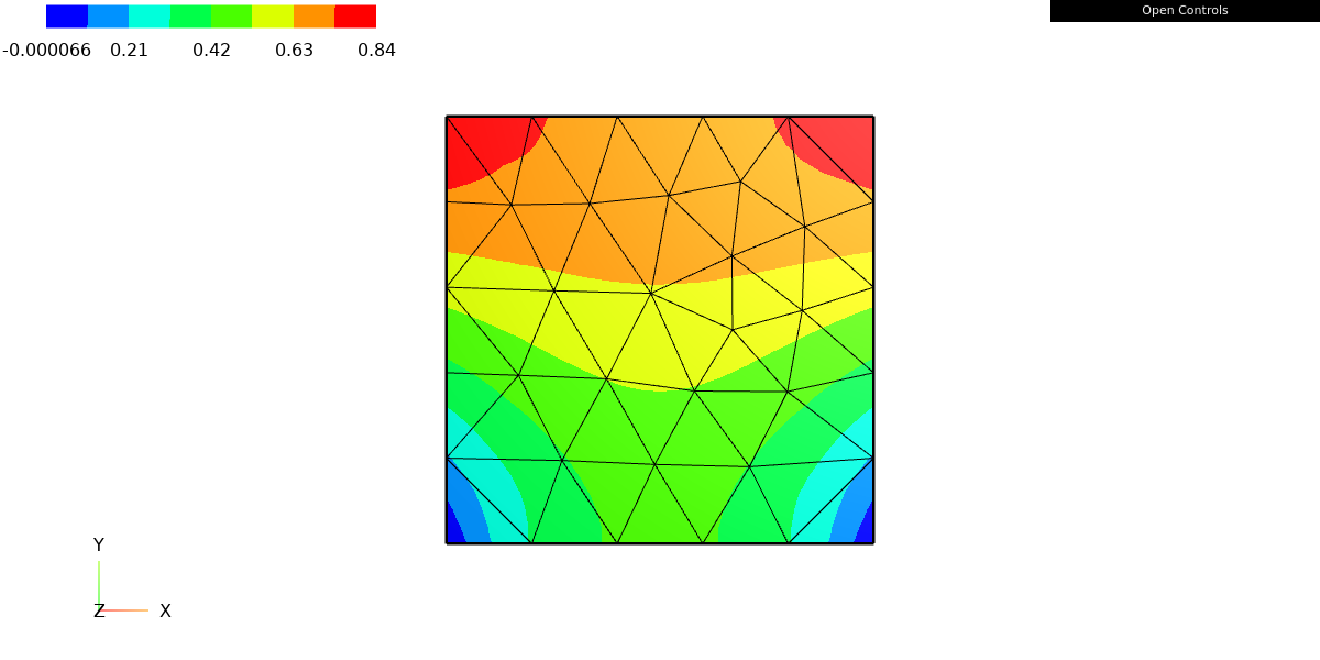
gfu.vec.data += a.mat.Inverse(freedofs=fes.FreeDofs()) * r
Draw(gfu)

This code updates the current value of the grid function gfu by adding the solution to the linear system represented by a.mat * gfu.vec = f.vec.

The first part of the operation a.mat.Inverse(freedofs=fes.FreeDofs()) computes the inverse of the assembled matrix of the bilinear form a, it is used to solve the linear system. freedofs=fes.FreeDofs() is used to specify that only the free degrees of freedom of the solution, which are not constrained by any condition, should be considered while solving the system. This can be useful in cases where some degrees of freedom are known and fixed.

The second part *r computes the product of the inverse matrix by the residual vector. This product represent the update of the solution.

Then the solution update is added to the current value of the grid function gfu.vec.data +=

Finally, the last line Draw(gfu) is used to visualize the updated solution. As it is mentioned before, it will open a window with the solution graph, assuming the required visualization library is installed.