6. Integrate a CoefficientFunction

Integrate(myfunc, mesh)

The Integrate function in ngsolve is used to compute the integral of a function over the domain of a given mesh. The function to be integrated is specified as a CoefficientFunction, and the mesh over which the integral is to be computed is specified as a Mesh object.

In this case, the Integrate function is being called with myfunc and mesh as arguments. This will compute the integral of myfunc over the domain represented by the mesh object.

The result of the Integrate function is a tuple of two values: the value of the integral and an estimate of the error in the integral. The error estimate is based on the number of quadrature points used to approximate the integral.

For example, if myfunc is the function f(x) = x*(1-x), then the integral of myfunc over the unit square is equal to 1/6. The Integrate function will return a tuple of the form (integral, error), where integral is the value of the integral and error is an estimate of the error in the integral.

You can use the Integrate function to compute integrals of functions defined on meshes in various dimensions, including 1D, 2D, and 3D meshes. You can also specify the integration order and the quadrature rule to be used.

7. Differentiate a CoefficientFunction

diff_myfunc = myfunc.Diff(x)
Draw(diff_myfunc, mesh, "derivative");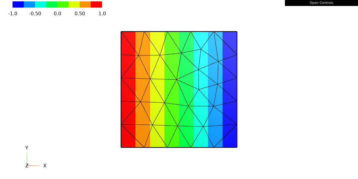

The Diff method of the CoefficientFunction class in ngsolve is used to compute the derivative of a function with respect to a given variable. The variable is specified as an argument to the Diff method.

In this case, the Diff method is being called with the global variable x as an argument. This will compute the derivative of myfunc with respect to x. The result is a new CoefficientFunction object that represents the derivative of myfunc. This object is stored in the diff_myfunc variable.

The Draw function is then called to visualize the derivative of myfunc. The Draw function is given three arguments:

• diff_myfunc: the CoefficientFunction to be plotted
• mesh: the Mesh object on which diff_myfunc is defined
• "derivative": a string specifying the name of the plot

This code will create a plot of the derivative of myfunc on the specified mesh, using the web-based graphical user interface (GUI) provided by ngsolve. The plot will be given the name “derivative”.

As before, you can view the plot by starting the ngsolve GUI server and opening the plot in a web browser using the Draw.GUI() function.

print(diff_myfunc)

he print function will print a string representation of the diff_myfunc object to the console. The string will contain the Python code that was used to create the object.

In this case, the print function will output the following string:

x*(-1) + (-x + 1)

This string represents the function f'(x) = -x + 1, which is the derivative of the function f(x) = x*(1-x).

You can use the print function to debug your code and to inspect the values of variables at different points in your program. You can also use the repr function to obtain a more detailed string representation of an object, which includes the object’s type and memory address. For example, print(repr(diff_myfunc)) will output a string that includes the type and memory address of the diff_myfunc object, in addition to its value.

8. Include parameter in CoefficientFunctions

k = Parameter(1.0)
f = sin(k*y)
Draw(f, mesh, "f");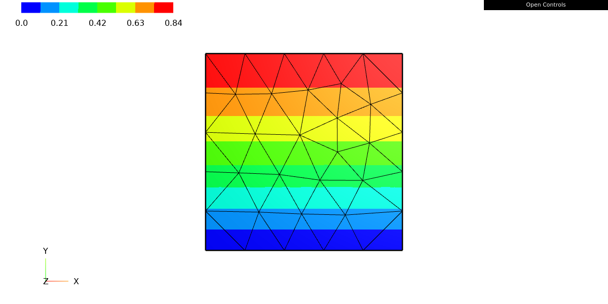

This code defines a Parameter object k with a value of 1.0, and a CoefficientFunction object f that represents the function f(y) = sin(ky). The Parameter class is used to represent variables that can be changed at runtime, and is often used to specify parameters in finite element simulations.

The Draw function is then called to visualize the function f on the mesh object. The Draw function is given three arguments:

• f: the CoefficientFunction to be plotted
• mesh: the Mesh object on which f is defined
• "f": a string specifying the name of the plot

This code will create a plot of the function f on the specified mesh, using the web-based graphical user interface (GUI) provided by ngsolve. The plot will be given the name “f”.

You can view the plot by starting the ngsolve GUI server and opening the plot in a web browser using the Draw.GUI() function.

You can change the value of the k parameter by assigning a new value to it. For example, you can set k=2.0 to update the function f to f(y) = sin(2y). The Draw function will update the plot to reflect the new value of k. This allows you to explore how the function f changes as the parameter k is varied.

k.Set(10)
Draw(f, mesh, "f");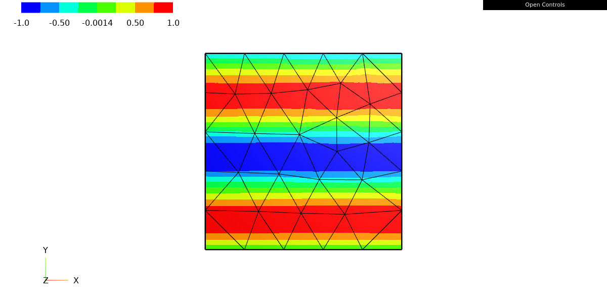

The Set method of the Parameter class is used to change the value of the parameter. In this case, the Set method is being called with the value 10 as an argument, which will change the value of the k parameter from its current value (1.0) to 10.0.

The Draw function is then called to update the plot of the function f, which depends on the value of the k parameter. The Draw function is given three arguments:

• f: the CoefficientFunction to be plotted
• mesh: the Mesh object on which f is defined
• "f": a string specifying the name of the plot

This code will update the plot of the function f to reflect the new value of the k parameter. The plot will be given the name “f”.

You can view the updated plot by starting the ngsolve GUI server and opening the plot in a web browser using the Draw.GUI() function.

The Set method allows you to change the value of the k parameter at runtime, which allows you to explore how the function f changes as the parameter is varied. You can use this feature to study the behavior of the function f under different conditions, or to optimize the function with respect to the parameter k.

print(f)

The print function will print a string representation of the f object to the console. The string will contain the Python code that was used to create the object.

In this case, the print function will output the following string:

sin(k*y)

This string represents the function f(y) = sin(ky), which depends on the value of the k parameter. The value of k is currently 10.0, so the function f is equal to f(y) = sin(10y).

You can use the print function to debug your code and to inspect the values of variables at different points in your program. You can also use the repr function to obtain a more detailed string representation of an object, which includes the object’s type and memory address. For example, print(repr(f)) will output a string that includes the type and memory address of the f object, in addition to its value.

print (f.Diff(k))

The Diff method of the CoefficientFunction class in ngsolve is used to compute the derivative of a function with respect to a given variable. The variable is specified as an argument to the Diff method.

In this case, the Diff method is being called with the k parameter as an argument. This will compute the derivative of f with respect to k. The result is a new CoefficientFunction object that represents the derivative of f with respect to k.

The print function will then print a string representation of the resulting object to the console. The string will contain the Python code that was used to create the object.

In this case, the print function will output the following string:

y*cos(k*y)

This string represents the function f'(k) = y*cos(ky), which is the derivative of the function f(y) = sin(ky) with respect to the parameter k.

You can use the Diff method to compute the derivatives of functions defined on meshes in various dimensions, including 1D, 2D, and 3D meshes. You can also specify the order of the derivative to be computed.

Integrate((f.Diff(k) - y*cos(k*y))**2, mesh)

The Integrate function in ngsolve is used to compute the integral of a function over the domain of a given mesh. The function to be integrated is specified as a CoefficientFunction, and the mesh over which the integral is to be computed is specified as a Mesh object.

In this case, the Integrate function is being called with an expression as an argument. The expression is the square of the difference between the derivative of f with respect to k and the function y*cos(k*y). The integral of this expression over the domain represented by the mesh object will be computed.

The result of the Integrate function is a tuple of two values: the value of the integral and an estimate of the error in the integral. The error estimate is based on the number of quadrature points used to approximate the integral.

This code will compute the integral of the squared difference between the derivative of f with respect to k and the function y*cos(k*y) over the domain represented by the mesh object. The value of the integral and the error estimate will be returned as a tuple.

You can use the Integrate function to compute integrals of functions defined on meshes in various dimensions, including 1D, 2D, and 3D meshes. You can also specify the integration order and the quadrature rule to be used.

9. Interpolate a CoefficientFunction into a finite element space

fes = H1(mesh, order=1)
u = GridFunction(fes)
u.Set(myfunc)
Draw(u);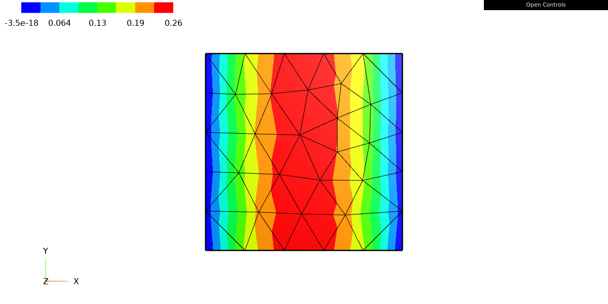

This code creates a finite element space fes of continuous, piecewise linear functions on the mesh object. The space is defined using the H1 class, which represents the standard Sobolev space of square-integrable functions with square-integrable first derivatives. The order argument specifies the order of the finite element basis functions, which in this case is 1 (linear basis functions).

A GridFunction object u is then created on the finite element space fes. The GridFunction class is used to represent functions defined on finite element spaces, and provides methods for evaluating the function at specific points, computing its integral and derivative, and visualizing the function.

The Set method of the GridFunction class is then called to set the value of the function u to the function myfunc. This assigns the values of myfunc to the degrees of freedom (DOFs) of the u function.

The Draw function is then called to visualize the function u on the mesh object. The Draw function is given one argument:

• u: the GridFunction to be plotted

This code will create a plot of the function u on the mesh object, using the web-based graphical user interface (GUI) provided by ngsolve. The plot will show the values of the function u at the nodes of the finite element mesh.

You can view the plot by starting the ngsolve GUI server and opening the plot in a web browser using the Draw.GUI() function.

You can use the GridFunction class to represent and manipulate functions defined on finite element spaces in ngsolve. You can use the Set method to set the values of the function, and the Draw function to visualize the function on a mesh. You can also use the Integrate and Norm methods to compute integrals and norms of the function, and the Deriv method to compute derivatives of the function.

10. Define vector-valued CoefficientFunctions,

vecfun = CoefficientFunction((-y, sin(x)))
Draw(vecfun, mesh, "vecfun");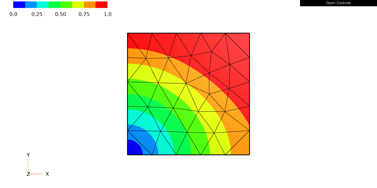

This code creates a CoefficientFunction object vecfun that represents a vector-valued function. The function is defined as a tuple of two functions: (-y, sin(x)), which represent the x- and y-components of the vector function, respectively.

The Draw function is then called to visualize the vector function vecfun on the mesh object. The Draw function is given three arguments:

• vecfun: the CoefficientFunction to be plotted
• mesh: the Mesh object on which vecfun is defined
• "vecfun": a string specifying the name of the plot

This code will create a plot of the vector function vecfun on the mesh object, using the web-based graphical user interface (GUI) provided by ngsolve. The plot will show the values of the vector function at the nodes of the mesh, using arrows to indicate the direction and magnitude of the vectors.

You can view the plot by starting the ngsolve GUI server and opening the plot in a web browser using the Draw.GUI() function.

You can use the CoefficientFunction class to represent and manipulate vector-valued functions in ngsolve. You can use the Draw function to visualize the function on a mesh, and you can use the Evaluate method to evaluate the function at specific points. You can also use the Diff method to compute derivatives of the function, and the Integrate method to compute integrals of the function.

u.Set(myfunc)
gradu = grad(u)
Draw(gradu, mesh, "grad_firstfun");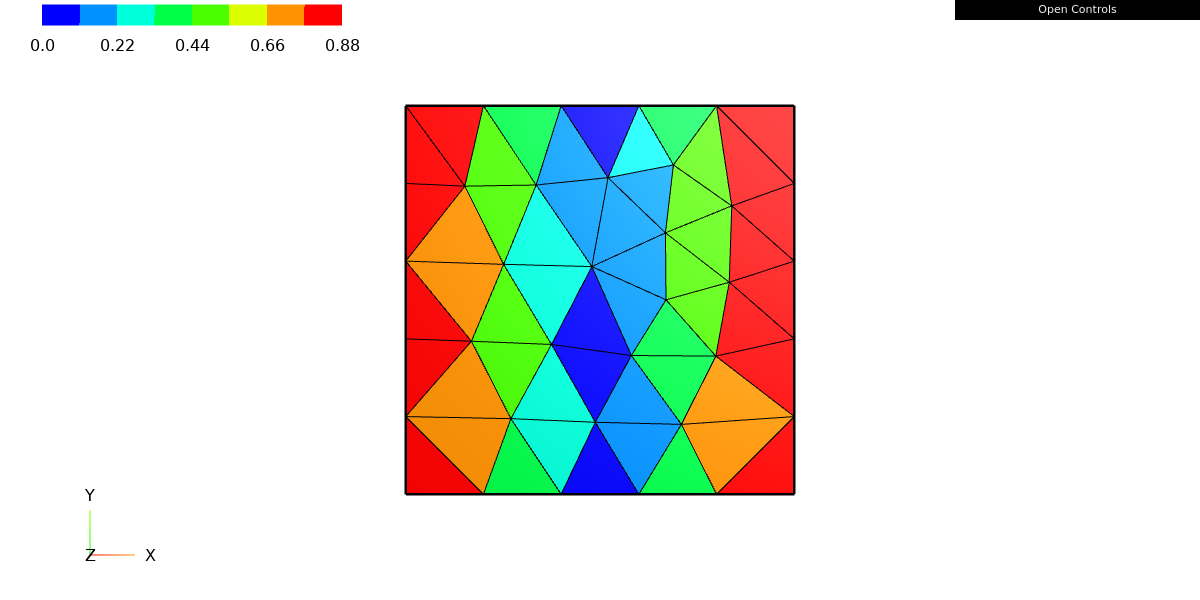

This code sets the value of the GridFunction u to the function myfunc using the Set method. The grad function is then called to compute the gradient of u, which is a vector-valued function that represents the derivative of u with respect to each spatial coordinate. The result is stored in the gradu variable.

The Draw function is then called to visualize the gradient of u on the mesh object. The Draw function is given three arguments:

• gradu: the gradient of u to be plotted
• mesh: the Mesh object on which gradu is defined
• "grad_firstfun": a string specifying the name of the plot

This code will create a plot of the gradient of u on the mesh object, using the web-based graphical user interface (GUI) provided by ngsolve. The plot will show the values of the gradient at the nodes of the mesh, using arrows to indicate the direction and magnitude of the vectors.

You can view the plot by starting the ngsolve GUI server and opening the plot in a web browser using the Draw.GUI() function.

11. Compile CoefficientFunctions

myfunc_compiled = myfunc.Compile()

The Compile method of the CoefficientFunction class in ngsolve is used to compile a function into machine code, which can be executed faster than the interpreted Python code. The compiled function is represented by a CF_Compiled object, which is a subclass of the CoefficientFunction class.

In this case, the Compile method is being called on the CoefficientFunction object myfunc. This will compile the function myfunc into machine code and return a CF_Compiled object that represents the compiled function. The compiled function is stored in the myfunc_compiled variable.

You can use the Compile method to improve the performance of your code by compiling functions that are called frequently or that are computationally intensive. The compiled function can then be used in the same way as the original function, using the same methods and functions.

Note that not all functions can be compiled, and the compilation process may fail if the function contains certain types of expressions or operations that are not supported by the compiler. In such cases, the Compile method will raise an exception. You can use the Compile method to test whether a function can be compiled, and to obtain more information about the compilation process.

f0 = myfunc
f1 = f0*y
f2 = f1*f1 + f1*f0 + f0*f0
f3 = f2*f2*f2*f0**2 + f0*f2**2 + f0**2 + f1**2 + f2**2
final = f3 + f3 + f3
finalc = final.Compile()

This code defines several CoefficientFunction objects: f0, f1, f2, f3, and final. These functions are defined by combining the function myfunc with itself and with other functions using arithmetic operations.

The final function is then compiled into machine code using the Compile method, and the resulting compiled function is stored in the finalc variable.

The finalc function is a CF_Compiled object, which is a subclass of the CoefficientFunction class. It represents the compiled version of the final function, which can be executed faster than the interpreted Python code.

You can use the Compile method to improve the performance of your code by compiling functions that are called frequently or that are computationally intensive. The compiled function can then be used in the same way as the original function, using the same methods and functions.

Note that not all functions can be compiled, and the compilation process may fail if the function contains certain types of expressions or operations that are not supported by the compiler. In such cases, the Compile method will raise an exception. You can use the Compile method to test whether a function can be compiled, and to obtain more information about the compilation process.

%timeit Integrate(final, mesh, order=10)

This code uses the timeit magic command to measure the execution time of the Integrate function. The Integrate function is called with the final function as an argument, and the order argument is set to 10 to specify the integration order. The mesh object is also passed as an argument to the Integrate function to specify the domain over which the integral is to be computed.

The timeit magic command will execute the Integrate function multiple times and return the average execution time. This can be useful for benchmarking the performance of your code and for comparing the execution time of different functions.

The timeit magic command takes one argument: the code to be executed. In this case, the argument is the Integrate function call.

You can use the timeit magic command to measure the execution time of any Python code. The timeit magic command is particularly useful for measuring the execution time of small pieces of code that are executed frequently or that are computationally intensive. It can be used to optimize the performance of your code and to identify bottlenecks in your program.

Note that the execution time measured by the timeit magic command is not necessarily representative of the overall performance of your program, as it does not take into account the time spent executing other parts of your code or the time spent waiting for external resources. It is intended as a rough guide to the execution time of the code being tested.

By comparing the execution times of the Integrate function with the final function and with the compiled finalc function, you can see the impact of compiling the function on its execution time. In general, compiled functions will execute faster than interpreted functions, but the improvement in performance will depend on the complexity and structure of the function being compiled.

finalcc = final.Compile(realcompile=True, wait=True)

This code calls the Compile method on the final function, with the realcompile and wait arguments set to True. The realcompile argument specifies that the function should be compiled using a standalone C++ compiler, rather than using the ngsolve JIT compiler. The wait argument specifies that the Compile method should block until the compilation process is complete.

The Compile method returns a CF_Compiled object that represents the compiled function. In this case, the compiled function is stored in the finalcc variable.

The realcompile argument can be used to specify that the function should be compiled using a standalone C++ compiler, rather than using the ngsolve JIT compiler. This can be useful if you want to produce a standalone executable that does not depend on the ngsolve library.

The wait argument can be used to specify that the Compile method should block until the compilation process is complete. This can be useful if you want to ensure that the compiled function is available for use before continuing with the execution of your code.

You can use the Compile method to improve the performance of your code by compiling functions that are called frequently or that are computationally intensive. The compiled function can then be used in the same way as the original function, using the same methods and functions.

Note that not all functions can be compiled, and the compilation process may fail if the function contains certain types of expressions or operations that are not supported by the compiler. In such cases, the Compile method will raise an exception. You can use the Compile method to test whether a function can be compiled, and to obtain more information about the compilation process.